It seems natural that if we take a random \(n\times n\) symmetric matrix then the
eigenvalues, which are generically \(n\) distinct real numbers, should be random
as well. Some naive experiments with matlab/octave can
surprise us revealing a strange form of randomness. For instance, if we
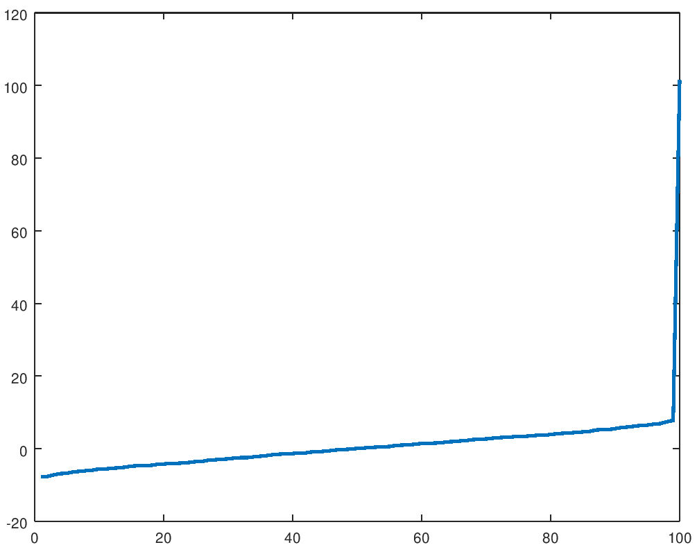
try A = rand(100) and plot( eig(A+A') ) then we
get typically a figure like this:
|
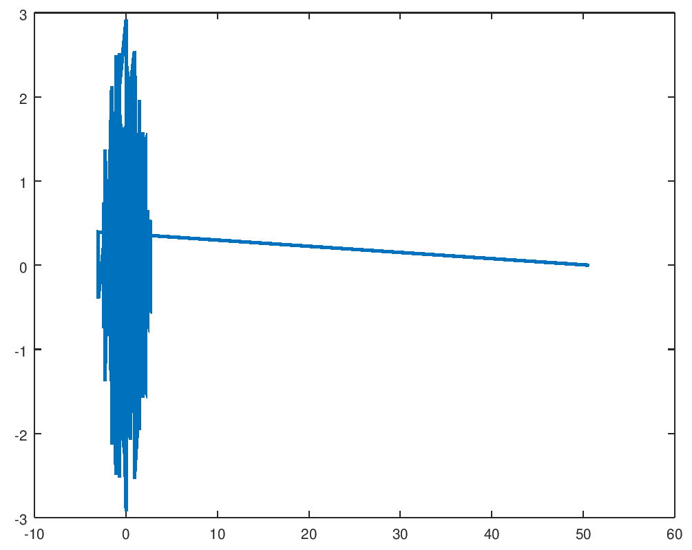
If we try simply plot( eig(A) ) to avoid any connection
with the symmetry, we obtain something like this:
 |
The explanation is simple. The rand command generates
pseudorandom numbers uniformly distributed in \((0,1)\). Then we can think that \(A=\frac{1}{2}\textbf{1}+B\) with \(\textbf{1}\) the matrix having all the
entries one while the entries of \(B\) are evenly distributed in \((-1/2,1/2)\). With
plot( eig(A-1/2*ones(100)) ) we check that \(B\) has the expected randomness:
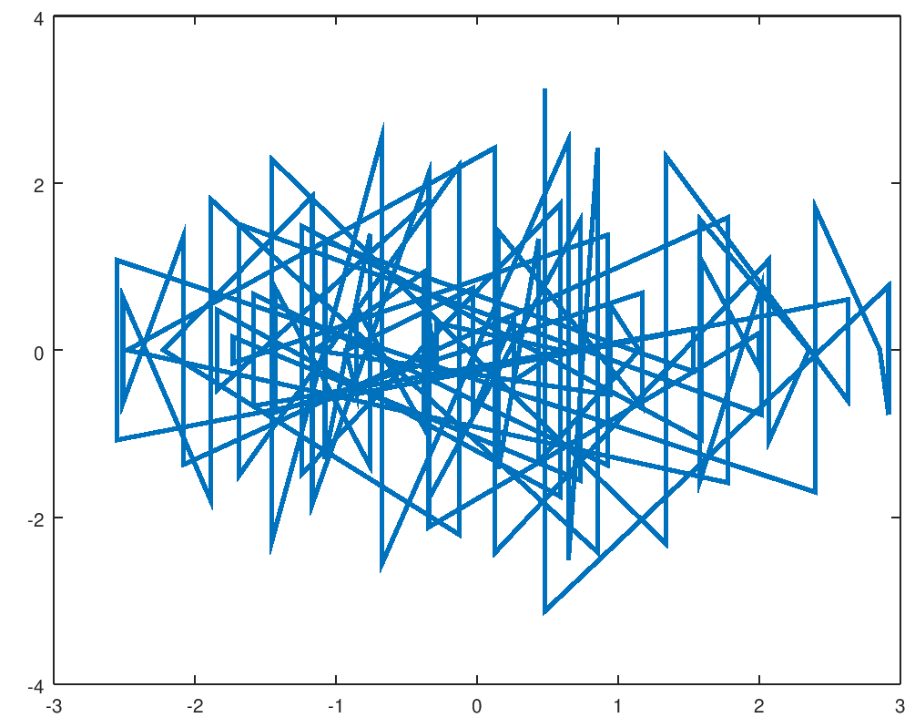 |
rand, we expect a large eigenvalue of size \(n/2\), in agreement with our previous
experiments.
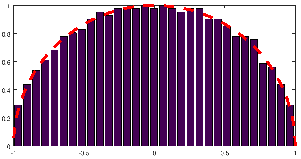
The loose end in the previous argument is that we are assuming that when the entries are uniformly distributed in \((-1/2,1/2)\) or, in general, in \((-a,a)\), the eigenvalues cannot be very large in comparison to \(n/2\) in the typical situations. The so called Wigner's semicircle law goes a step forward in the case of symmetric (or Hermitian) matrices and shows that under quite general conditions, there is a limiting distribution for the scaled eigenvalues. The usual proofs are based on computing the moments using the trace of powers of the matrix. This idea is in early works of E. P. Wigner who firstly stated a result of this kind (see for instance this for a more general mathematical statement). The plot of the density function of the limiting distribution is a semicircle after scaling (i.e., a semiellipse). By this reason, the probability distributions having this property are called Wigner semicircle distribution.
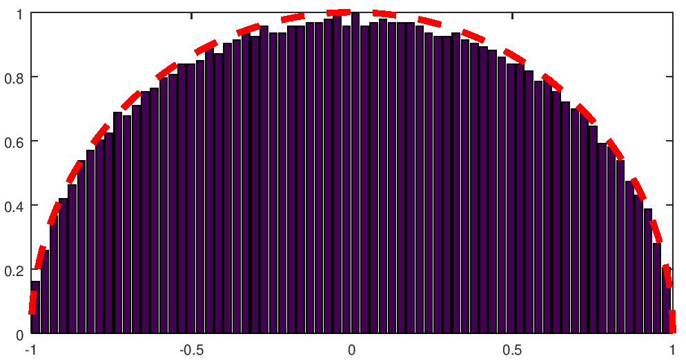
The matlab/octave code below creates a symmetric matrix with independent entries (except for the symmetry) uniformly distributed in \((-1,1)\) and plots the histogram of the eigenvalues conveniently scaled to fit in \([-1,1]\times [0,1]\).
Running it we get figures like this:
 |
N = 1000 |
To see the semicircle, the dimension must be large. Even 100 is too small, as the following figure shows. Other experiments with the same dimension give worse results.
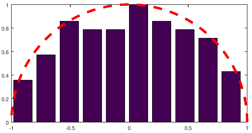 |
N = 100 |
Increasing the dimension to 5000 and the number of bins as the square root, we do not see fundamental improvements.
 |
N = 5000 |
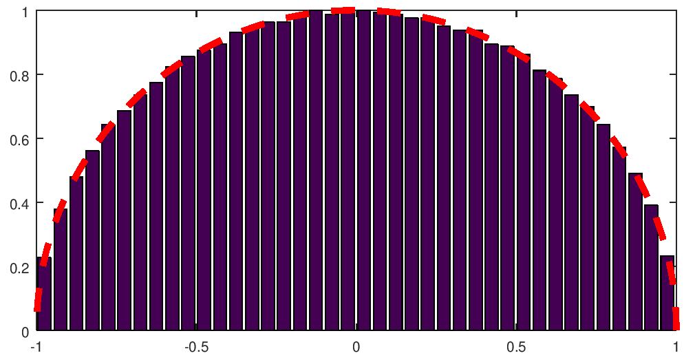 |
N = 5000 |
The result does not depend on the distribution of the entries (under
mild conditions). For instance, we could change the third line by
A = randn(N), which use a standard Gaussian distribution,
without any sensible effect.
matlab/octave to make the images showing the semicircular histograms.
% Random symmetric matrix |