When monochromatic coherent light passes through a diffraction grating, the diffraction pattern replicates the structure of the grating at distances given by integral multiples of certain length, the Talbot length, while at fractional multiples one gets shifted or scaled copies of this structure. In general terms, this phenomenon is called the Talbot effect because it was firstly vaguely mentioned by H. F. Talbot in a purely descriptive paper published in 1836 about early experiments on diffraction. Many years later, in 1881, Lord Rayleigh (J. W. Strutt) wrote "On copying diffraction-gratings..." including a theoretical explanation.
The plane diagram combining the 1D diffraction wave intensity patterns at each distance is called the Talbot carpet and it possesses a fractal-like looking structure. Observing real optical Talbot carpets (as well as many other diffraction light phenomena) is not easy. However, a classroom experiment can be devised to visualize the Talbot effect with water waves. Here we show images of artificial Talbot carpets based on the exponential sums coming from diffraction theory that are usually introduced to explain the phenomenon. The images have been generated with the matlab/octave code below (there is also a not very advisable older sagemath version).
Let us consider the slits in a periodic diffraction grating as holes at integers values of the \(Y\)-axis. If a monochromatic plane wave of frequency \(\nu\) and wavelength \(\lambda\ll 1\) enters the diffraction grating from the left half plane, each hole acts as a source of a spherical wave (Huygens-Fresnel principle) and, using the abbreviation \(e(x)=e^{2\pi ix}\), we can model the diffracted wave as \[u(\mathbf{x},t)= \sum_{\mathbf{k}} e\big(\mathbf{k}\cdot \mathbf{x}-\nu t\big) \qquad\text{with}\quad |\mathbf{k}|=\lambda^{-1}\text{ and }k_2\in\mathbb{Z}.\] Here \(\mathbf{k}\) is the wave vector as used in crystallography and it differs in a factor \(2\pi\) from the standard one in physics. The condition \(k_2\in\mathbb{Z}\) comes from the grating equation.
In reality, the slits in the grating have certain width \(w\) and there are many sources of close interacting waves. According to Fraunhofer diffraction, the waves in the preceding sum are affected by the Fourier transform of the characteristic function of an interval (the sinc function). Then, the theoretical diffraction intensity pattern corresponds to the square of \[F(x,y)= |u(x,y,t)|= \bigg| \sum_{|n|\le \lambda^{-1}} \frac{\sin(n\pi w)}{n\pi} e\big(x\sqrt{\lambda^{-2}-n^2}+ny\big) \bigg|.\]
The usual explanation of the Talbot effect is that the main contribution to the sum comes from small values of \(n\) and the paraxial approximation of the geometrical optics suggests that we can substitute the square root for its first order Taylor expansion in \(n^2\). After this substitution, \(u(x,y,t)e(-\lambda^{-1} x)\) and \(u(x+2\lambda^{-1},y,t)\) are close and we see a periodicity in the diffraction pattern for distances differing in integral multiples of the Talbot length \(2\lambda^{-1}\). For the case of fractional multiples, we have to take into account the cancellation encoded in the quadratic Gauss sums, which gives a nice relation to number theory.
From the physical perspective, it is natural to consider a density plot of \(F^2\) (related to the intensity) rather than of \(F\), but it is visually less appealing. In fact, depending on your taste, plotting \(F^\alpha\) with \(0\lt\alpha\lt 1\) could give more information. In the following, we plot \(F\) all the time. This has nothing to do with Physics, it is more like the histogram equalization in image processing. An aesthetic point is that we use the jet color map (instead of a grayscale) in which blue is for small values and red for larger ones (see a graphic table of several color maps at the end of this page in the Matlab documentation).
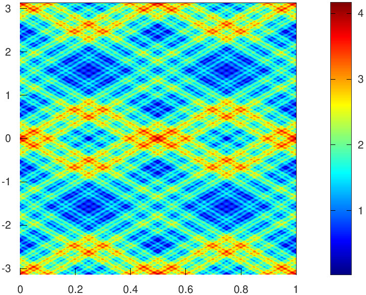
Our basic example is:
|
| \(\lambda^{-1}=100\), \(w=0.1\), resolution 300 |
The resolution mentioned in the caption is the number of nodes in the \(X\) and \(Y\) axes to do the evaluations. This means that there are 90000 evaluations of \(F\).
If we change the sinc window function in \(F\) by another with exponential decay, the result is in practice as the superposition of few waves, but one still distinguishes the same structure in the Talbot carpet.
 |
| Window \(= w\exp(-\pi^2 w^2 x^2)\) with \(w=0.1\) |
Recovering the original sinc window, if \(w\) is decreased, then we have a superposition of many waves and the result tends to be more homogeneous. Usually, we see mainly a blue background because we have very large invisible isolated peaks.
In the following figure corresponding to \(w=0.03\), to avoid the shift of the colormap due to their contribution and observe a less monotone Talbot carpet, we only plot here the points in which the value is below 80% of the maximum.
 |
| \(\lambda^{-1}=100\), \(w=0.03\) |
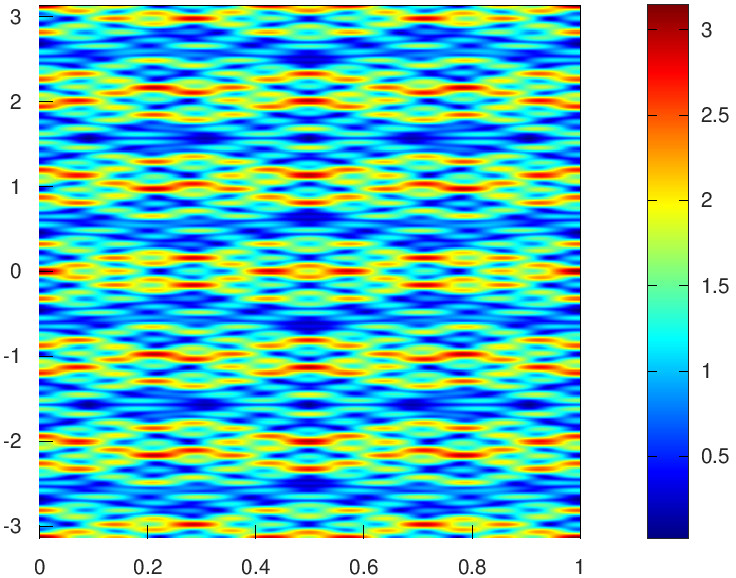
Let us increase the value of \(w\) equating in the modeled diffraction the width of the slits and the separation between then. It corresponds to the Ronchi grating. In this case, \(F\) is more wave like because in the sum we do not have highly oscillation terms with noticeable relative amplitude which could give an approximation to rays in their interference. The plot is in this case:
 |
| \(\lambda^{-1}=100\), \(w=0.5\) |
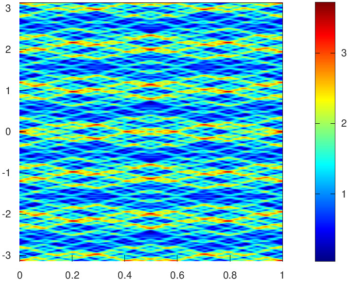
If \(w^{-1}\) is not much smaller than \(\lambda^{-1}\) then the assumptions of the paraxial approximation are not fulfilled. This is an example with very low frequency:
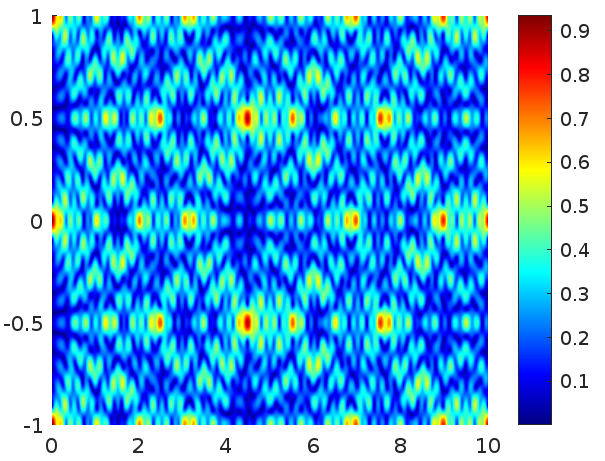 |
| \(\lambda^{-1}=5\), \(w=0.1\) |
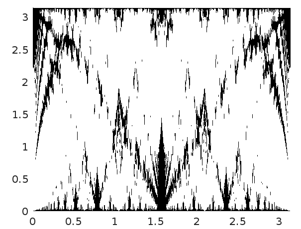
The points at which \(F\) is very small from what is called here, in a related setting, the "valleys of the shadows". The following figure shows in black the points with values smaller than 10% of the maximum.
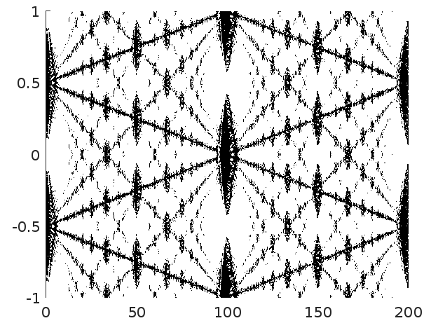 |
| \(\lambda^{-1}=100\), \(w=0.1\), resolution 500 |
The related setting mentioned in the last paragraph corresponds to the density plots of solutions of the Schrödinger equation. This is called the quantum Talbot effect. The axes of the carpet are time and position. For a circle or a sphere, the Talbot effect considered as a periodicity in time is trivial, as well as in any example with commensurable energy levels. In a broader context this is named quantum revival.
We focus on the example of the sphere, the solution of \[i\frac{\partial\Psi}{\partial t} = -\nabla^2_{S^2}\Psi \qquad\text{with}\quad \Psi(\theta,0)=f_r(\theta)\] where \(f_r\) is a certain regular function depending on the parameter \(0<r<1\) and \(|f_r|^2\) tend to the Dirac \(\delta\) at the north pole of the sphere as \(r\to 1^-\). Here, as usual, \(\theta\) is the polar angle.
Namely, we define for \(0<r<1\) \[f_r(\theta)=c_rF(r,\theta) \qquad\text{with}\quad F(r,\theta)= \frac{1}{\sqrt{(r-\cos\theta)^2+\sin^2\theta}} \qquad\text{and}\quad c_r = \Big( \frac{2\pi}{r}\log\frac{1+r}{1-r} \Big)^{-1/2} .\] A calculation proves that it is normalized as a function on the sphere: \[\int_{S^2} |f_r|^2 = 2\pi \int_0^\pi \big|f_r(\theta)\big|^2 \sin\theta\, d\theta=1.\] Note that \(c_r\to 0\) and \(f_r(\theta)\) remains bounded when \(r\to 1^-\) and \(0<\theta\le\pi\). Then \(|f_r|^2\) tends to the Dirac delta on the north pole of the sphere. As a matter of fact, these calculations are very similar to those showing that the Poisson kernel is an approximation of the identity.
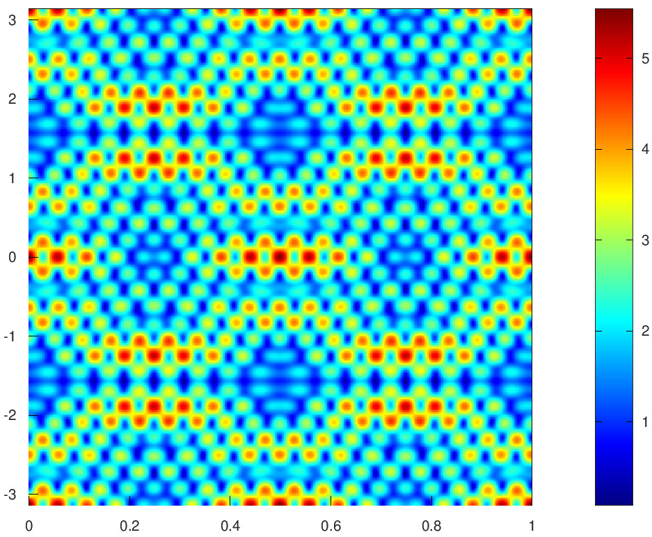
This is the quantum Talbot carpet corresponding to plot the square root of \(|\Psi(\theta,t)|^2\sin\theta\) for \(r=0.95\). The horizontal axis represents time and the vertical axis represents polar angle. The value of \(N\) is the number of terms employed in the eigenfunction expansion. Experimentally, taking it higher does not change substantially the result for this choice of \(r\). Values of \(r\) closer to 1 require more terms in the eigenfunction expansion.
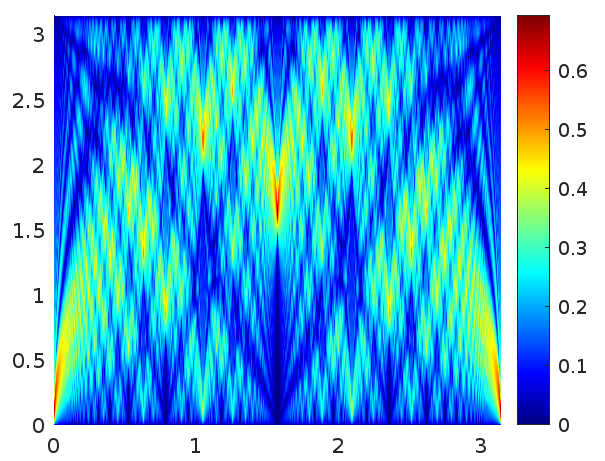 |
| \(r=0.95\), \(N=1000\) |
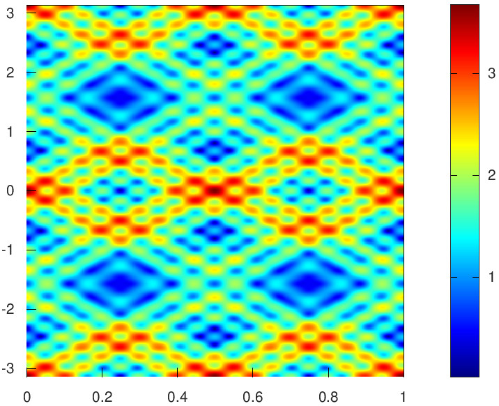
If \(r\) is reduced, the peaks are not so sharp, as this figure reveals:
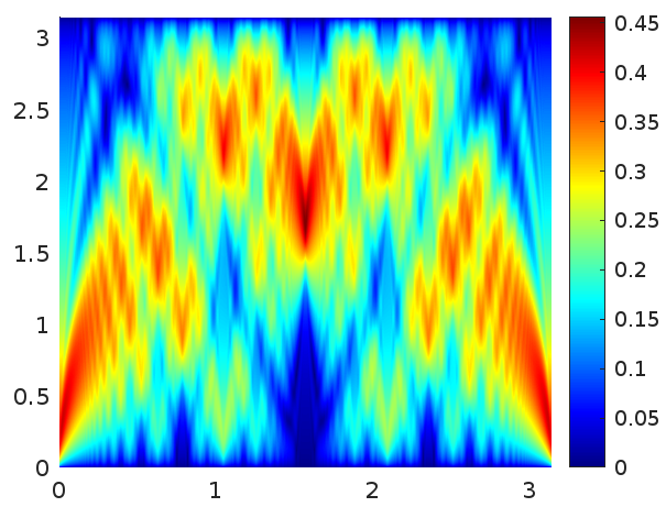 |
| \(r=0.8\), \(N=1000\) |
For the case \(r=0.95\), these are the "valleys of the shadows" corresponding to points with values smaller than 15% of the maximum.
 |
| \(r=0.95\), \(N=1000\) |
Consider particles confined in a flat torus obtained identifying the opposite sides of \[[2\pi R_1, 0]\times [0, 2\pi R_2]\times\{0\}.\] In this situation the cartesian coordinates may be parameterized as \(x=R_1\phi_1\), \(y=R_2\phi_2\), \(z=0\) with \(\phi_1\) and \(\phi_2\) two \(2\pi\)-periodic angles. For a fermionic particle ruled by Dirac equation the plane wave solutions are of the form \[\Psi_{\vec{n}} = \frac{1}{\sqrt{2}} \bigg( 1+\frac{q}{\sqrt{\vec{n}^2+q^2}} \bigg)^{1/2} \begin{pmatrix} 1 \\ 0 \\ 0 \\ \frac{n_1+in_2}{q+\sqrt{\vec{n}^2+q^2}} \end{pmatrix} e^{i(n_1\phi_1+n_2\phi_2-\sqrt{\vec{n}^2+q^2}\, c t/R)},\] where \[q=\frac{McR}{\hbar}.\] The 1-dimensional case corresponds to set \(n_1=0\) (so, the state does not depend on \(\phi_1\)) and the \(2\)-dimensional case to leave it free.
Up to a rotation, a generic state having a discrete, finite and nonnegative energy spectrum is a superposition of the form \[\Phi = \sum_{\vec{n}\in\mathcal{N}}\lambda_{\vec{n}} \Psi_{\vec{n}} \qquad\text{with}\quad \lambda_{\vec{n}}\in\mathbb{C}-\{0\}\] where \(\mathcal{N}=\big\{\vec{n}_0,\vec{n}_1,\dots, \vec{n}_N\big\}\), \(\vec{n}_j=(k_j,l_j)\in\mathbb{Z}^2\) and \(k_j=0\) in the one dimensional model. The energy spectrum is related to the squared norm of the \(\vec{n}_j\). It is the set \[\mathcal{E} = \Big\{ \frac{c\hbar}{R} \sqrt{k_j^2+\ell_j^2+q^2}\,:\, (k_j,\ell_j)\in\mathcal{N} \Big\}.\] We want to characterize the possible sets \(\mathcal{N}\) containing \(\vec{n}_0\) such that quantum revivals appear. More concretely, given \(\vec{n}_0\) we want to determine the maximal set of quantum numbers \(\mathcal{N}_0\) including \(\vec{n}_0\), such that \(\Phi\) is periodic in \(t\) if and only if \(\mathcal{N}\) is a finite subset of \(\mathcal{N}_0\).
The set \(\mathcal{N}_0\) is infinite if and only if \(q^2\in\mathbb{Q}\) except for \(\ell_0^2+q^2\) being a square in the 1-dimensional case.
Let us start with a 1D example having a finite \(\mathcal{N}_0\). Consider \(\ell_0=3\) and \(q=\frac 32 \sqrt{21}\). Then \[\mathcal{N}_0 = \big\{ (0,\pm3), (0,\pm5), (0,\pm15), (0,\pm47) \big\}.\] The corresponding carpet is:
 |
| Full \(\mathcal{N}_0\) with \(\lambda_{\vec{n}}=1\). |
| Matlab/Octave generating code |
 |
| \(\mathcal{N}_0-\{(0,\pm 47)\}\) with \(\lambda_{\vec{n}}=1\). |
| Matlab/Octave generating code |
For \(\ell_0=5\), \(q=\sqrt{2}\) it can be proved \[\mathcal{N}_0 = \big\{ (0,\pm c_n)\text{ where } \ell_{n+1}=4\ell_{n}-\ell_{n-1} \text{ with } \ell_{-1}=1,\ \ell_0=5 \big\}.\] Due to the exponential growth of \(\ell_n\), even for fairly small cardinalities of \(\mathcal{N}\), the state \(\Phi\) shows large variations for tiny changes of \(\phi_2\) and \(t\) and the density plot is close to be a cloud of random points. In this context it is natural to let \(\lambda_{\vec{n}}\) to decay with \(|\vec{n}|\).
This is the result choosing the six \(\ell_j\) with smallest absolute values and \(\lambda_{\vec{n}}=|\vec{n}|^{-1/4}=|\ell_j|^{-1/4}\).
 |
| \(\ell_j=\pm1,\pm5,\pm19\), \(\lambda_{\vec{n}}=|\ell_j|^{-1/4}\). |
| Matlab/Octave generating code |
 |
| \(\ell_j=\pm1,\pm5,\pm19,\pm71\), \(\lambda_{\vec{n}}=|\ell_j|^{-1/4}\). |
| Matlab/Octave generating code |
To mask the light cones, a possibility is to take \(q^2\) large to avoid \(\sqrt{\ell_j^2+q^2}/|\ell_j|\) to be close to 1, at least for the first values of \(\ell_j\). With this idea in mind consider the example \(\vec{n}_0=(0,3)\) and \(q=\sqrt{791}\).
With six values of \(\ell_j\) it is obtained
 |
| \(\ell_j=\pm3,\pm19,\pm39\), \(q^2=791\). |
| Matlab/Octave generating code |
 |
| \(\ell_j=\pm3,\pm19,\pm39,\pm71\), \(q^2=791\). |
| Matlab/Octave generating code |
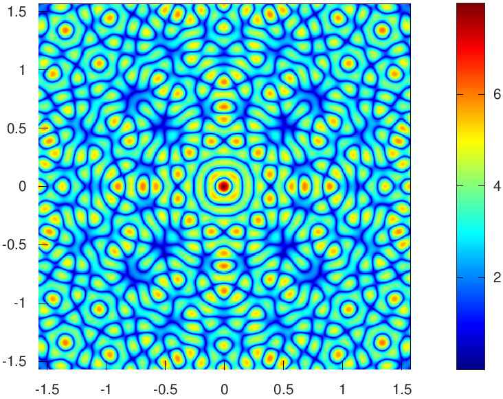
This is a plot of the nodal lines of the first coordinate of the state \(\Phi\) for \(\mathcal{N}_0\) with \(k_0^2+\ell_0^2=1105\), \(q^2\not\in\mathbb{Q}\) and \(\lambda_{\vec{n}}=1\) in the range \(\phi_1,\phi_2\in [-\pi/2,\pi/2]\).
 |
| Nodal lines \(k_0^2+\ell_0^2=1105\), \(\lambda_{\vec{n}}=1\). |
| Matlab/Octave generating code |
This is the corresponding density plot of \(|\Phi|^{0.5}\). As \(e^{-iEt/\hbar}\) is constant, \(|\Phi|\) does not depend on \(t\). The exponent \(0.5\) is only for visualization purposes. It has been introduced to mollify the effect of the peak at \(\phi_1=\phi_2=0\).
 |
| \(|\Phi(\phi_1,\phi_2)|^{0.5}\), \(\lambda_{\vec{n}}=1\). |
| Matlab/Octave generating code |
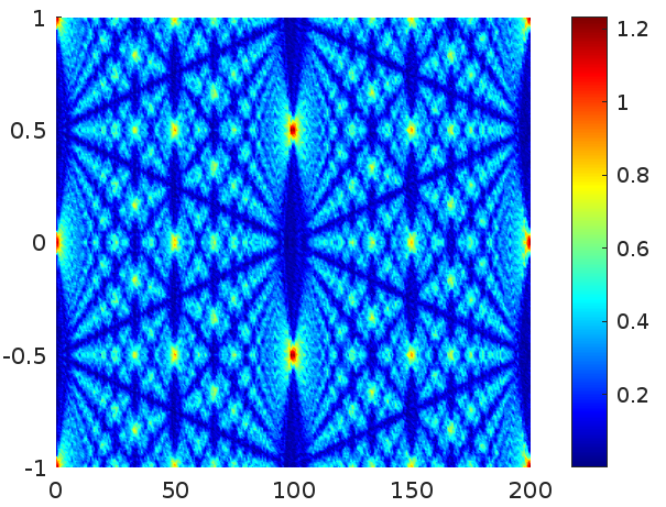
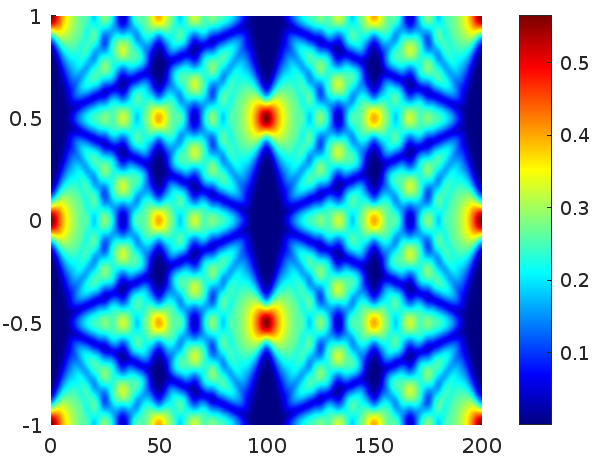
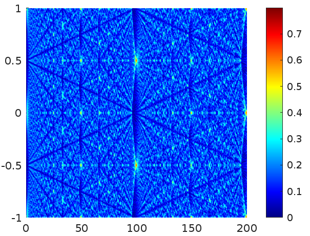
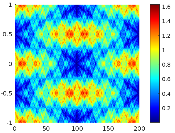
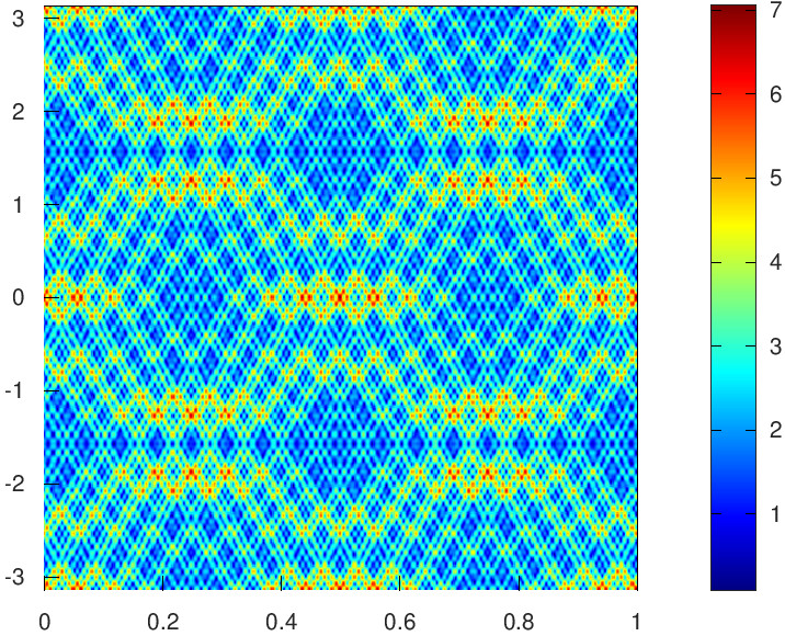
Consider now the example \((k_0,\ell_0)=(1,2)\) with \(q^2=3\) and take \[\mathcal{N}= \big\{ (\pm1,\pm2),\, (\pm2,\pm1),\, (\pm2,\pm5),\, (\pm5,\pm2),\, (\pm2,\pm11),\, (\pm11,\pm2),\, (\pm5,\pm10),\, (\pm10,\pm5) \big\}.\] The density plot of the associated state \(\Phi\) is not feasible because there are three variables \((\phi_1,\phi_2,t)\). To illustrate the situation, the following figure is composed by \(4\) images showing the density plots in \((\phi_1,\phi_2)\) for \(t=0,\, T_{\text{\rm rev}}/10,\, T_{\text{\rm rev}}/5\) and \(T_{\text{\rm rev}}/10\).
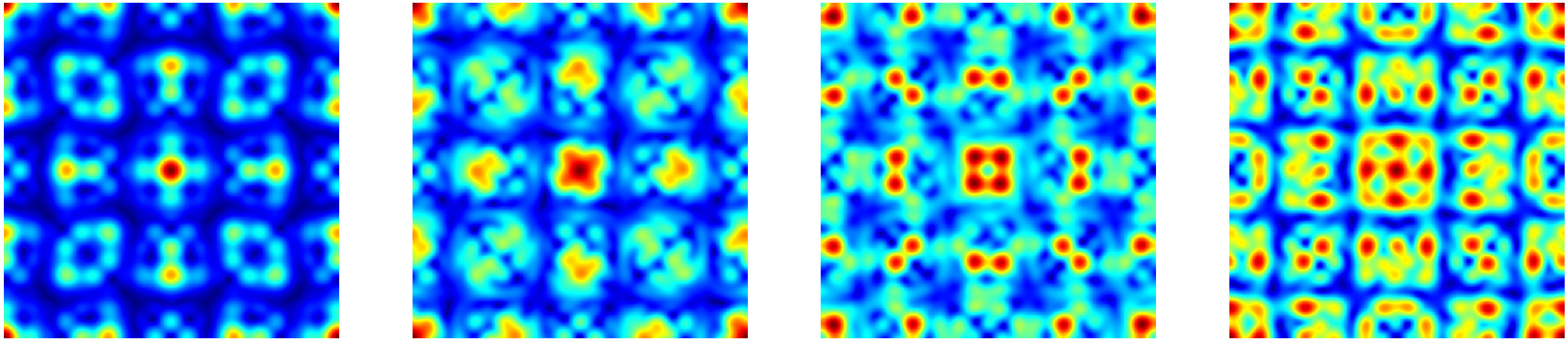 |
| \(|\Phi(\phi_1,\phi_2,kT_{\text{\rm rev}}/10)|\) for \(k=0,1,2,3\), \(\phi_1,\phi_2\in [-\pi,\pi]\), with \(\lambda_{\vec{n}}=1\). |
| Matlab/Octave generating code |
The linked codes have been tested with Octave in https://sagecell.sagemath.org/.
|
function [X,Y,R] = density_F( linv, wf, pr, tol) |
|
function [TH,T,R] = density_FQ( r, N, NT, tol) |
plot_carpet commands took
677.6+667.5+676.2+2724+669.3+2623+1451+665.1
seconds, this makes a little less than 3 hours.
import time |