There exists a simple and nice algorithm to find an optimal coding for a finite space of probability (a finite set of symbols and their probabilities or frequencies). Here optimal means that it gives the minimal average length. One of the reasons to say that it is “nice” is that for small sets we can carry out the algorithm by hand constructing a tree, in the sense of graph theory, starting from the leaves. For the algorithm and its properties see the Wikipedia or any book covering a minimum of information theory.
Given a table of frequencies (or probabilities) this code displays the Huffman coding and plots the corresponding tree. Namely, the output of the function huf_tre is a list of pairs frequency-encoding and a graph. Actually if we are only interested in the list we can use a direct call to huf_cod instead.
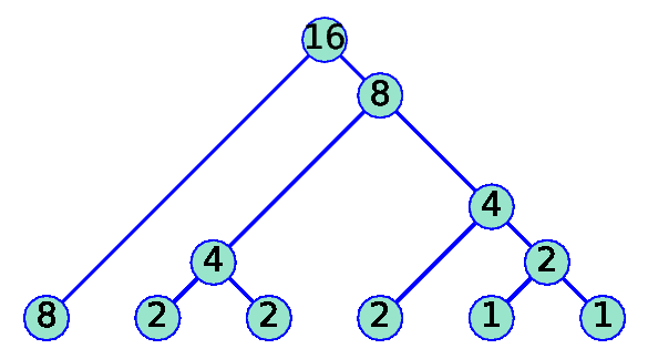
As an example of the simplest use, with LP = huf_tre( [8, 2, 2, 2, 1, 1] ) we obtain in LP[0] the list [(8, '0'), (2, '100'), (2, '101'), (2, '110'), (1, '1110'), (1, '1111')] and LP[1] is the figure
|
Besides the required list of frequencies, huf_tre admits two optional arguments. The first is boolean and indicates if we want to see the codification in the figure. For instance, if in the previous case we write huf_tre( [8, 2, 2, 2, 1, 1], True ) then the figure becomes
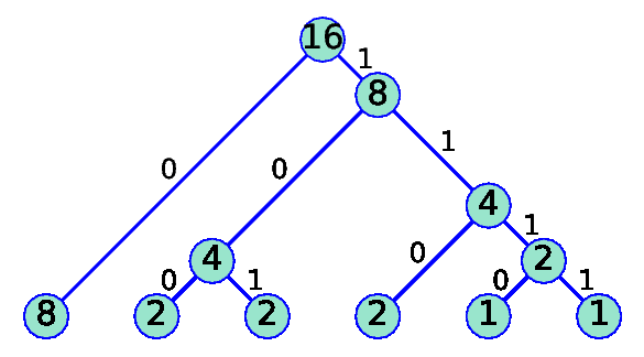 |
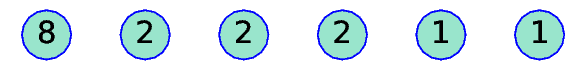
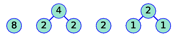
The second optional argument indicates the number of iterations in the Huffman algorithm if we want to see an intermediate forest (the set of subtrees at a certain step). Moreover, there are plotting parameters (defined in the code after the function huf_cod) that can be configured. For instance, h is the base separation of the leaves. Changing the value of rci to h/4 and running a for loop in which k takes the values 0, 1, 2, 3, 4, 5 we have the following sequence of figures showing how the tree is formed:
k=0 |
 |
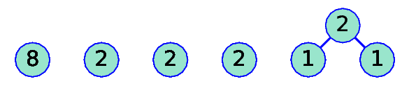
k=1 |
 |
k=2 |
 |
k=3 |
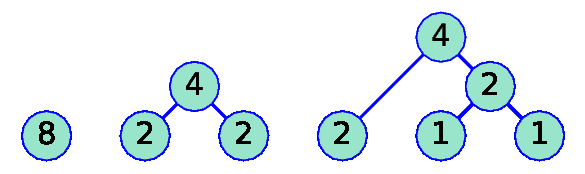 |
k=4 |
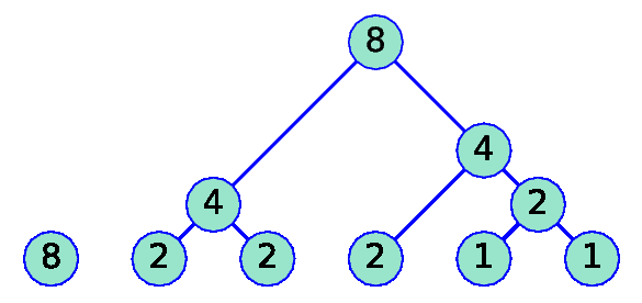 |
k=5 |
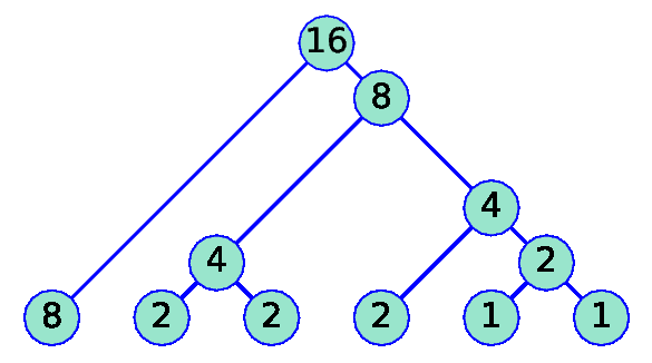 |
To give a last example on the possibility of playing with the parameters, setting the aspect ratio with ar = 0.7, the font size with fs = 12 and the font size to radii of the circles with rci = h/4, we get running huf_tre( [1/2, 1/8, 1/8, 1/8, 1/16, 1/16] )
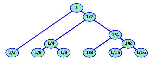 |
This is SAGE code that gives the codification and the tree of the Huffman coding.
def add_nodes( N1, N2 ):

  N3 = [ N1[0]+N2[0], [] ]

  for item in N1[1]:

    N3[1].append( (item[0], '0'+item[1]) )

  for item in N2[1]:

    N3[1].append( (item[0], '1'+item[1]) )

  return N3


def huf_cod ( Lprob ):

  """

  Input: list of frequencies or probabilities

  Output: reordered list of frequencies and

    their corresponding enconding (lexicographic order)

  """

  LN = [ [item,[(item,'')]] for item in Lprob ]


  while len(LN)>1:

    # The lambda is to choose always the first

    N1 = min(LN, key=lambda nn: nn[0])

    LN.remove( N1 )

    N2 = min(LN, key=lambda nn: nn[0])

    LN.remove( N2 )

    LN.append( add_nodes(N1,N2) )


  L = LN[0][1][:]

  # not necessary?

  L.sort(key=lambda nn: nn[1])

  return L


# separation nodes

h = 1

# node circles color

cico = (0.6,0.9,0.8)

# text color

teco = 'black'

# thickness

th = 2

# fontsize

fs = 22

# fontsize 0 and 1

fs01 = 18

# aspect ratio

ar = 1


# node circles radius

rci = h/5

#offset 0 and 1

ho01 = h*fs01/300


def plot_circ_node( nod ):

  P = circle( nod[2], rci, fill=True, facecolor= cico, zorder=10)

  P += text( str(nod[0]), nod[2], fontsize =fs, color = teco, zorder=20)

  return P


def joint_two_nodes( node1, node2, cod ):

  if node1[2][0] > node2[2][0]:

    node1, node2 = node2, node1

  x1,y1 = node1[2]

  x2,y2 = node2[2]

  x3,y3 = (x1+x2+y2-y1)/2, (-x1+x2+y2+y1)/2

  node3 = [ node1[0]+node2[0] , node1[1][:-1], ( x3, y3 )]

  Q = line( [node1[2], node3[2], node2[2]], thickness=th )

  Q += plot_circ_node( node3 )

  if cod:

    Q += text( '1', ((x2+x3)/2+ho01,(y2+y3)/2+ho01), horizontal_alignment='left', fontsize =fs01, color = teco)

    Q += text( '0', ((x1+x3)/2-ho01,(y1+y3)/2+ho01), horizontal_alignment='right', fontsize =fs01, color = teco)

  return node3, Q


def init_nodes( Lprob ):

  Lnodes = []

  P = point( [(0,0)], size=0)

  for k in range( len(Lprob) ):

    nnode = [Lprob[k][0], Lprob[k][1], (k*h,0)]

    P += plot_circ_node( nnode )

    Lnodes.append( nnode )

  return Lnodes, P


def huf_tre( Lprob, cod =False, niter=-1 ):

  """

  Input: list of frequencies or probabilities

    optional:   codification True or False

          number of iterations

  Output: Plot of the Huffman tree

  """

  Lcodif = huf_cod(Lprob)

  Lnodes, P = init_nodes( Lcodif )

  # The call to huf_cod is for the right ordering

  if niter==-1: niter += len( Lprob )

  for k in range(niter):

    # The lambda is to choose always the first

    node1 = max(Lnodes, key=lambda nn: len(nn[1]) )

    Lnodes.remove( node1 )

    pref = node1[1][:-1]

    for item in Lnodes:

      if item[1][:-1] == pref:

        node2 = item

        break

    Lnodes.remove( node2 )

    node3, Q = joint_two_nodes( node1, node2, cod )

    Lnodes.append( node3 )

    P += P+Q


  P.axes(False)

  P.fontsize(16)

  P.set_aspect_ratio(ar)

  return Lcodif, P


################

# EXAMPLE 1

# (default)

LP = huf_tre( [8, 2, 2, 2, 1, 1] )

print LP[0]

LP[1].save('./file.eps', figsize = 6)


################

# EXAMPLE 2 codif.

# (default)

LP = huf_tre( [8, 2, 2, 2, 1, 1], True )

print LP[0]

LP[1].save('./file.eps', figsize = 6)


################

# EXAMPLE 3

# (with rci = h/4)

for k in range(6):

  LP = huf_tre( [8, 2, 2, 2, 1, 1], False, k )

#  LP[1].save('./file'+str(k)+'.eps', figsize = 6)

print LP[0]


################

# EXAMPLE 4

# (with ar = 0.7, fs = 12, rci = h/4)

LP = huf_tre( [1/2, 1/8, 1/8, 1/8, 1/16, 1/16] )

print LP[0]

LP[1].save('./file.eps', figsize = 6)