A fundamental pinch

The fundamental solution of the wave equation with initial zero velocity in a compact Riemannian manifold is

where the lambda's are the increasingly ordered distinct eigenvalues of the Laplace-Beltrami operator, the phi's are the corresponding normalized eigenfunctions and x₀ is the point of the manifold where the mass of the Dirac delta lies at. The index m and the (finite) summation on it regards the possibility of multiple eigenvalues for the same eigenvalue (degeneracy).

In the case of the unit sphere with the usual Euclidean metric we have exact and simple formulas for the eigenvalues and also exact (but not so simple) expressions for the eigenfunctions, they are the real spherical harmonics. This formula only makes sense when considered as a distribution because at the initial time it is the Dirac delta and the wave equation does not smooth data as opposed to the heat equation.
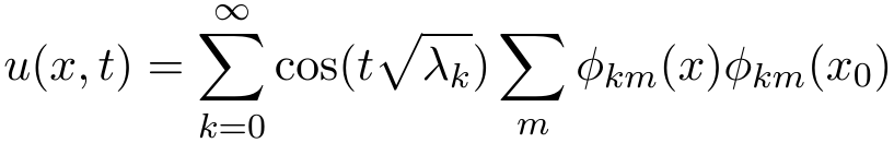
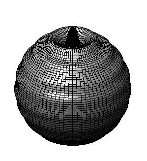
If we truncate the series, then for t=0 we obtain a peak approximating the Dirac delta. The wave equation gives an approximation of how vibrations evolve, then we can considered the truncated solution as an approximation of the evolution of a pinch applied on a elastic sphere. Here we show the figures of the numerical results. The scale of the pinch in terms of the radius has been adjusted to get a better visual effect. For details, check the matlab code at the end of this page.

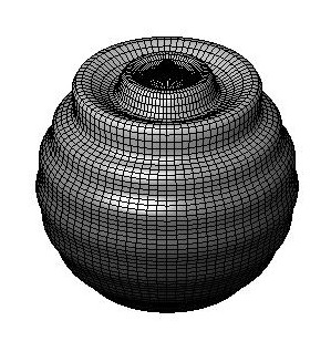
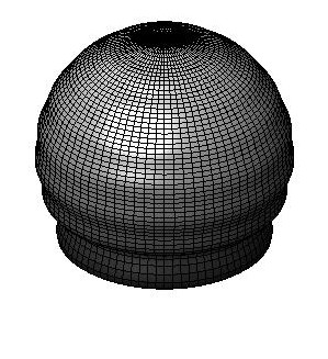
If you pinch a rubber sphere the first reaction is a quick and severe rebound:


`t = 0.0000`	`t = 0.1257`	`t = 0.2513`	`t = 0.3770`

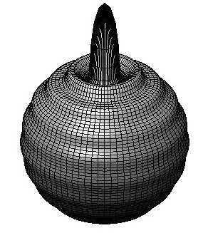
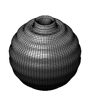
In the last image a "lump" shows up but with lesser strength because part of the energy escapes with the huge wavefront surrounding it.
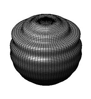
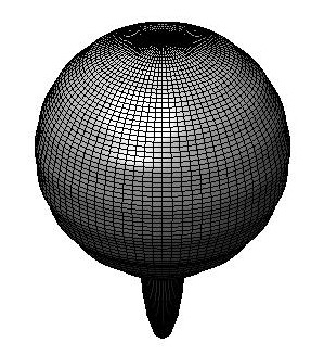
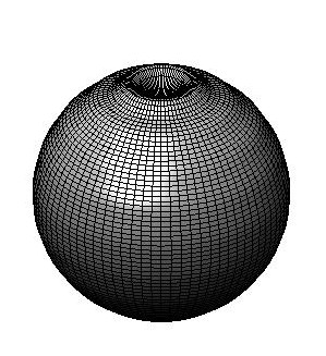
This an other wavefronts travel towards the south pole producing "love handles" on the sphere.


`t = 0.6283`	`t = 1.0053`	`t = 1.3823`	`t = 1.7593`

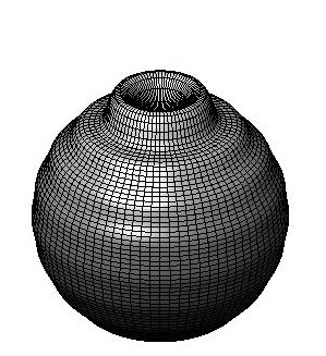
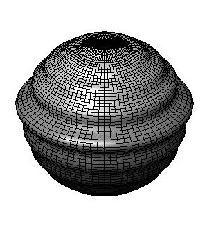
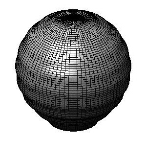
The waves interfere in the south pole to give a negative pinch that rebounds. Note that the pinch and the rebound occurs at a time close to pi, reflecting the fact that waves travel with speed one.


`t = 2.2619`	`t = 2.6389`	`t = 3.0159`	`t = 3.3929`

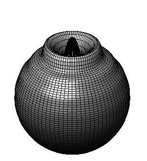
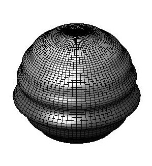
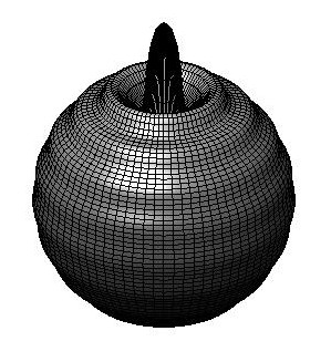
As expected, the waves come back to the north pole giving a north pinch.
After the works of Colin de Verdière, Chazarain and Duistermaat and Guillemin, we know that in general the trace has a singular support contained in the integer multiples of the length of the geodesics. This sounds natural in our case, because due to the symmetry the trace should be as sitting on the north pole and measuring the amplitude there for each time (analytically, one can appeal to the spherical harmonic addition theorem and the normalization P_l(1)=1). The rationale is that we have to wait 2*pi, the length of a meridian, to notice the same peak because the waves travel with speed one. On the other hand, the trace for the truncated series is a simple exponential sum and the frequencies (the square roots of the eigenvalues) are close to k+1/2 for large values of k. Hence one should observe negative peaks at odd multiples of 2*pi. This can be difficult to observe in the previous figures because the rebound is very quick. Let us see the last instants before t=2*pi with a small step:


`t = 6.0947`	`t = 6.1575`	`t = 6.2204`	`t = 6.2832`

Although analytically is clear, I do not see a geometric reason for this change in the phase when the time is increased by 2*pi, specially when one compares the situation with the 1D case corresponding to the unit circle. Note also that by the same analytic reason, at t=pi the peak should be negligible at the south pole because cos(t(k+1/2)) becomes close to zero.

The code

The matlab code used to generate the images is:
[Note: I confess that I realized too late that the spherical harmonic addition theorem, or the symmetry if you prefer, allows to write a simpler and much faster program. I keep this code because I want to do also some experiments with other particular solutions of the wave equation under other non-symmetric initial conditions].



      nframes = 51

      maxl = 20

      scale = 0.85;

      

      res = [80,80];

      

      phi = linspace(0,2*pi,res(1));

      theta = linspace(0, pi,res(2)); 

      [phi,theta] = meshgrid(phi,theta);

      

      

      for k = 0:nframes-1

          t = 2*pi*k/(nframes-1)

          S = ones(res)/sqrt(4*pi); % sum. The initial
      value is Y00

          for l=1:maxl

                  [k,l]

       
          P = legendre(l,cos(theta));

        
          for m=-l:l

                  
         %--compute Y_{lm}

                 
          Plm = squeeze(P(abs(m)+1,:,:));

                 
          base = sqrt(
      ((2*l+1)/(2*pi))*factorial(l-abs(m))/factorial(l+abs(m)) )*Plm;

                 
          if m>0

                 
              Ylm = base.*cos(m*phi);

                 
          elseif m == 0

                 
              Ylm = base/sqrt(2.0);

                 
          else

                 
              Ylm = base.*sin(-m*phi);

                 
          end

                  
         %-----

      

                 
          S = S + Ylm*Ylm(1,1)*cos(t*sqrt(l*(l+1)));

              end

          end

      

          rho = 1 + scale*S*12.0/maxl/maxl;

      

          %
https://es.mathworks.com/help/matlab/examples/animating-a-surface.html

          r = rho.*sin(theta); % convert to Cartesian
      coordinates

          x = r.*cos(phi);

          y = r.*sin(phi);

          z = rho.*cos(theta);

      

          figure(1)

          s = surf(x,y,z);

          colormap gray

          camlight right; lighting gouraud

          % camlight right; lighting phong

          view([40,30])

          camzoom(1.5)

          axis ([-3 3 -3 3 -3 3])

          axis off

          namefig = './images/sph%d_%d.jpg';

          namefig = sprintf(namefig,maxl,k);

          saveas(gcf,namefig)

          pause(1)

      end

Some obvious variations apply to generate short time variation around 0 and 2*pi.